
Streudiagramme Teil 6
Im Streudiagramm erkennt man durch das Muster der Punkte Informationen über die Abhängigkeitsstruktur der beiden Merkmale.
Stand: 27.04.2021
import matplotlib.pyplot as plt
import numpy as np
from pandas.plotting import scatter_matrix
#df['logarithm'] = np.log(df['Temperatur'])
#dfny = df.dropna()
#scatter_matrix(df['logarithm'])
#df.plot.scatter(df, loglog=True)
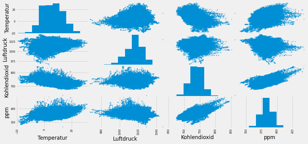
scatter_matrix(df_wasserkuppedrop, figsize=(15,7))
array([[<AxesSubplot:xlabel='Temperatur', ylabel='Temperatur'>,
        <AxesSubplot:xlabel='Luftdruck', ylabel='Temperatur'>,
        <AxesSubplot:xlabel='Kohlendioxid', ylabel='Temperatur'>,
        <AxesSubplot:xlabel='ppm', ylabel='Temperatur'>],
       [<AxesSubplot:xlabel='Temperatur', ylabel='Luftdruck'>,
        <AxesSubplot:xlabel='Luftdruck', ylabel='Luftdruck'>,
        <AxesSubplot:xlabel='Kohlendioxid', ylabel='Luftdruck'>,
        <AxesSubplot:xlabel='ppm', ylabel='Luftdruck'>],
       [<AxesSubplot:xlabel='Temperatur', ylabel='Kohlendioxid'>,
        <AxesSubplot:xlabel='Luftdruck', ylabel='Kohlendioxid'>,
        <AxesSubplot:xlabel='Kohlendioxid', ylabel='Kohlendioxid'>,
        <AxesSubplot:xlabel='ppm', ylabel='Kohlendioxid'>],
       [<AxesSubplot:xlabel='Temperatur', ylabel='ppm'>,
        <AxesSubplot:xlabel='Luftdruck', ylabel='ppm'>,
        <AxesSubplot:xlabel='Kohlendioxid', ylabel='ppm'>,
        <AxesSubplot:xlabel='ppm', ylabel='ppm'>]], dtype=object)
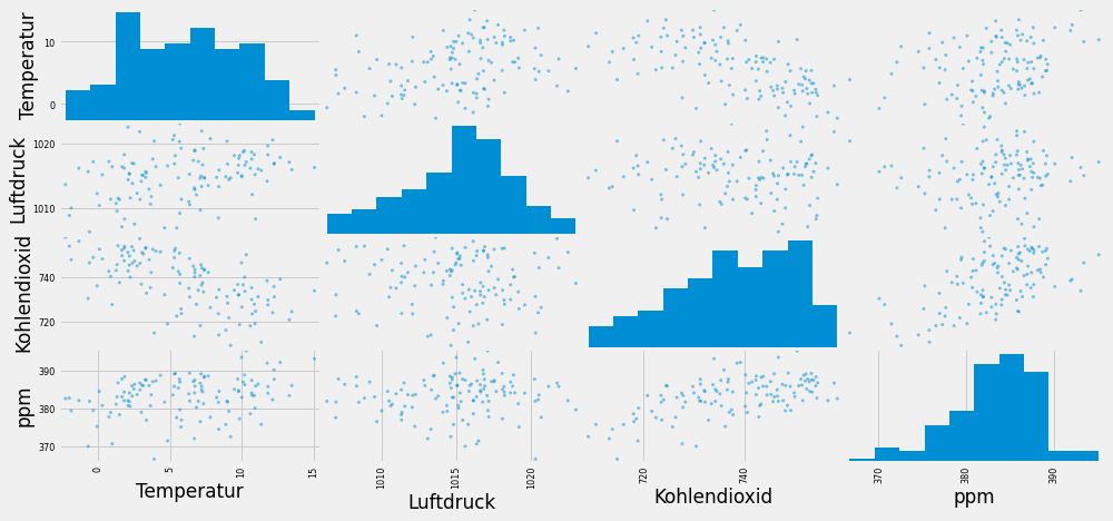
dfco2m = dfco2m.drop(columns = ['MA3'])
dfco2m
| Temperatur | Luftdruck | Kohlendioxid | ppm | |
|---|---|---|---|---|
| Datum | ||||
| 2011-01-31 | 9.861905 | 1018.083333 | 718.535714 | 377.267934 |
| 2011-02-28 | 10.933333 | 1015.166667 | 718.979167 | 380.087965 |
| 2011-03-31 | 10.738542 | 1012.093750 | 723.416667 | 383.434028 |
| 2011-04-30 | 10.977660 | 1008.351064 | 724.648936 | 385.891135 |
| 2011-05-31 | 8.386458 | 1008.500000 | 723.479167 | 381.627605 |
| ... | ... | ... | ... | ... |
| 2020-08-31 | 5.670833 | 1020.233333 | 751.100000 | 387.711256 |
| 2020-09-30 | 7.174167 | 1014.941667 | 745.800000 | 389.088071 |
| 2020-10-31 | 5.693333 | 1009.225000 | 741.425000 | 386.948444 |
| 2020-11-30 | 2.715833 | 1012.291667 | 745.200000 | 383.644441 |
| 2020-12-31 | 2.384167 | 1013.800000 | 746.466667 | 383.237839 |
120 rows × 4 columns
import matplotlib.pyplot as plt
import numpy as np
from pandas.plotting import scatter_matrix
#df['logarithm'] = np.log(df['Temperatur'])
#dfny = df.dropna()
#scatter_matrix(df['logarithm'])

#df.plot.scatter(df, loglog=True)

scatter_matrix(dfco2m , figsize=(15,7))
array([[<AxesSubplot:xlabel='Temperatur', ylabel='Temperatur'>,
        <AxesSubplot:xlabel='Luftdruck', ylabel='Temperatur'>,
        <AxesSubplot:xlabel='Kohlendioxid', ylabel='Temperatur'>,
        <AxesSubplot:xlabel='ppm', ylabel='Temperatur'>],
       [<AxesSubplot:xlabel='Temperatur', ylabel='Luftdruck'>,
        <AxesSubplot:xlabel='Luftdruck', ylabel='Luftdruck'>,
        <AxesSubplot:xlabel='Kohlendioxid', ylabel='Luftdruck'>,
        <AxesSubplot:xlabel='ppm', ylabel='Luftdruck'>],
       [<AxesSubplot:xlabel='Temperatur', ylabel='Kohlendioxid'>,
        <AxesSubplot:xlabel='Luftdruck', ylabel='Kohlendioxid'>,
        <AxesSubplot:xlabel='Kohlendioxid', ylabel='Kohlendioxid'>,
        <AxesSubplot:xlabel='ppm', ylabel='Kohlendioxid'>],
       [<AxesSubplot:xlabel='Temperatur', ylabel='ppm'>,
        <AxesSubplot:xlabel='Luftdruck', ylabel='ppm'>,
        <AxesSubplot:xlabel='Kohlendioxid', ylabel='ppm'>,
        <AxesSubplot:xlabel='ppm', ylabel='ppm'>]], dtype=object)
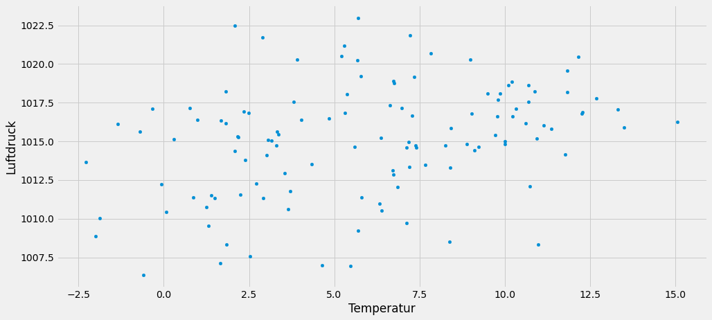
dfco2m.plot.scatter(x='Temperatur', y='Luftdruck', loglog=False, alpha=1, figsize=(15,7))
plt.show()
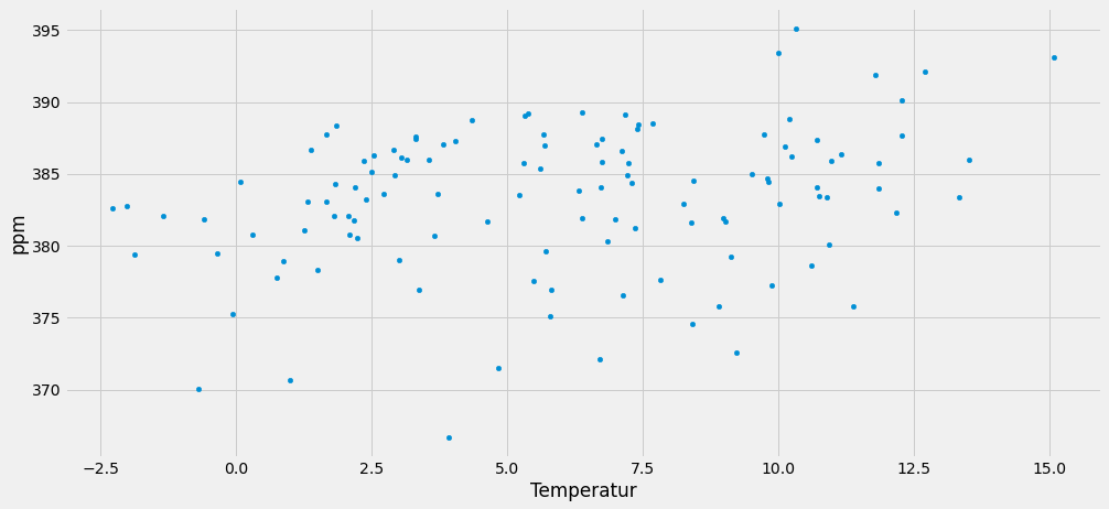
dfco2m.plot.scatter(x='Temperatur', y='ppm', loglog=False, alpha=1, figsize=(15,7))
plt.show()
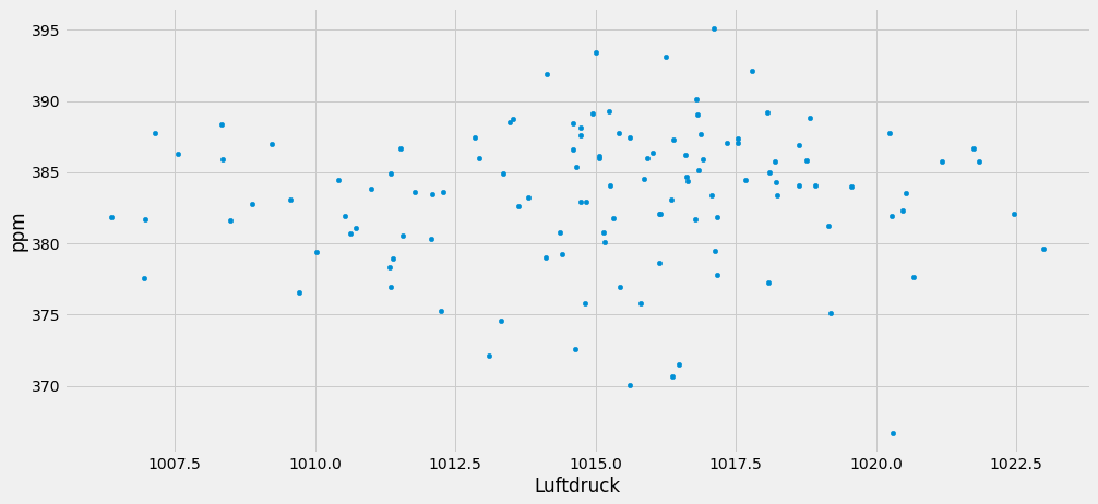
dfco2m.plot.scatter(x='Luftdruck', y='ppm', loglog=False, alpha=1, figsize=(15,7))
plt.show()
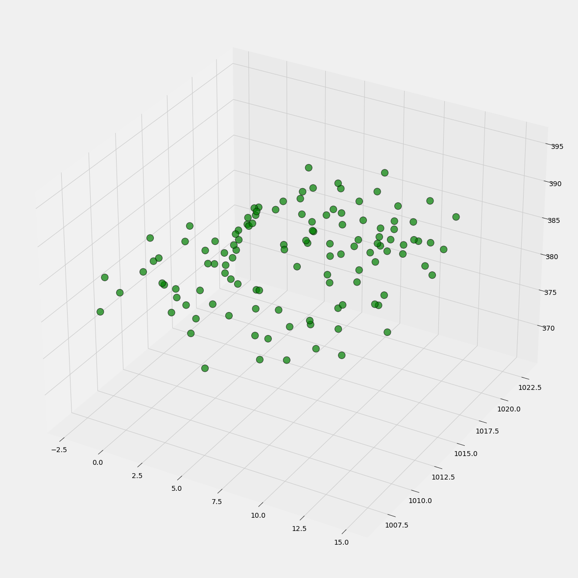
3D Streudiagramm
#https://stackoverflow.com/questions/59232073/scatter-plot-with-3-variables-in-matplotlib

#https://www.advsofteng.com/doc/cdpydoc/threedscatter2.htm Dropline


import matplotlib.pyplot as plt
from mpl_toolkits.mplot3d import Axes3D
import numpy as np

x = np.array(dfco2m['Temperatur'])
y = np.array(dfco2m['Luftdruck'])
z = np.array(dfco2m['ppm'])

fig = plt.figure(figsize=(20, 20))
ax = fig.add_subplot(111, projection='3d')
ax.scatter(x, y, z,
           linewidths=1, alpha=.7,
           edgecolor='k',
           s = 200,
           c='green',
           )
plt.show()
dfco2m.info()
<class 'pandas.core.frame.DataFrame'>
DatetimeIndex: 120 entries, 2011-01-31 to 2020-12-31
Freq: M
Data columns (total 4 columns):
 #   Column        Non-Null Count  Dtype
---  ------        --------------  -----
 0   Temperatur    120 non-null    float64
 1   Luftdruck     120 non-null    float64
 2   Kohlendioxid  120 non-null    float64
 3   ppm           120 non-null    float64
dtypes: float64(4)
memory usage: 4.7 KB
x.shape
(120,)
y.shape
(120,)
z.shape
(120,)
ToDO: Droplines https://matplotlib.org/devdocs/gallery/mplot3d/stem3d_demo.html
Siehe: https://support.minitab.com/de-de/minitab/19/help-and-how-to/graphs/3d-scatterplot/interpret-the-results/key-results/